I came across a tidy ecommerce sales dataset — 5,000 orders, 12 columns, no missing values. It’s the kind of file that looks ready to model at first glance, so before any of that I ran the numbers to see what it actually contains. Here’s the dataset, the walkthrough, and a few honest caveats.
The dataset
| Column | Type | Notes |
|---|---|---|
order_id |
int | Sequential, 10001–15000 |
order_date |
date | One order per day (US format m/d/Y) |
customer_id |
int | 989 unique customers |
product_category |
str | Electronics, Clothing, Home, Beauty |
region |
str | North, South, East, West |
quantity |
int | 1–10 |
unit_price |
float | |
discount |
float | 0–0.5, mean 0.18 |
payment_method |
str | Card, COD, Wallet |
delivery_days |
int | Mean 6.1 days |
customer_rating |
float | 1.0–5.0, mean 2.97 |
revenue |
float | Pre-computed line total |
📥 Download the CSV (341 KB, 5,000 rows).
What the data says
Revenue totals $5.1M across the four categories, with Electronics the clear leader:
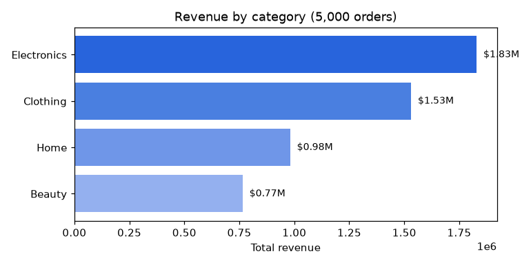
- Electronics: $1.83M (36%)
- Clothing: $1.53M (30%)
- Home: $0.98M (19%)
- Beauty: $0.77M (15%)
Regions are almost perfectly balanced (24–26% of revenue each), so there’s no regional story in this file. Card is the dominant payment method (45% of orders), followed by COD (35%) and Wallet (19%).
Revenue is driven by price and quantity, not service. Correlations with revenue: unit price +0.68, quantity +0.62, discount −0.14, delivery days +0.01, customer rating +0.01. Delivery speed and customer ratings have essentially no relationship with how much a basket is worth.
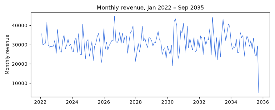
The monthly trend is flat — and suspiciously so:
The caveats
Before treating this as a real-world sample, a few things stand out:
- It’s synthetic. Dates run from 1 Jan 2022 to 9 Sep 2035 with exactly one order per day (5,000 orders / 365 days ≈ 13.7 years, leap years included). Real retailers get hundreds of orders a day, not one.
revenueis internally consistent — it’s exactlyquantity × unit_price × (1 − discount)on all 5,000 rows. That’s handy if you want to rebuild the column from the raw inputs, but it also means the file gives you no surprises there.- Ratings cluster oddly — 80 orders rated 1.0 and only 73 rated 5.0, with a roughly uniform distribution between. Real ratings are usually bimodal (happy vs. unhappy).
- The long time span with no growth makes any time-series forecast a flat line. Fine for practising pipelines, misleading if you want a seasonal story.
Good for
- Practising pandas EDA and data-cleaning workflows
- SQL exercises (aggregations, window functions, cohort analysis)
- Building dashboards before you have real data
- Testing forecasting pipelines where you expect no trend
Not great for: drawing conclusions about actual ecommerce behaviour. Treat it as a well-formed dataset for practising mechanics — not as evidence.
📥 Prefer the raw file? Download the CSV — 5,000 rows, ready for pandas or SQL.